Homepage Animation Tutorial

This notebook will cover the generation of the homepage animation. To run this notebook, please first generate the forcing fields by running all cells in idealized_fields.ipynb and generate the ray tracing output by running all cells in canonical_ray_tracing.ipynb.

# data handling
import xarray as xr
import numpy as np

# plotting
import matplotlib.pyplot as plt
import matplotlib.animation as animation
import cmocean
from IPython.display import HTML
from matplotlib.animation import PillowWriter

Setup

First, we open the forcing field datasets to use as the background of the animation.

zonal_jet = xr.open_dataset('./forcing/zonal_jet.nc')
eddy = xr.open_dataset('./forcing/mesoscale_eddy.nc')
island = xr.open_dataset('./forcing/gaussian_island.nc')
beach = xr.open_dataset('./forcing/gentle_slope.nc')

We then open the ray tracing bundles that were generated in canonical_ray_tracing.ipynb.

bundle4jet = xr.open_dataset('./output/bundle4zonal_jet.nc')
bundle4eddy = xr.open_dataset('./output/bundle4eddy.nc')
bundle4island = xr.open_dataset('./output/bundle4island.nc')
bundle4beach = xr.open_dataset('./output/bundle4beach.nc')

For the two examples of rays passing through canonical current fields, we calculate the current speed for the background.

zonal_speed = np.sqrt(zonal_jet.u**2 + zonal_jet.v**2)
eddy_speed = np.sqrt(eddy.u**2 + eddy.v**2)

We convert the x and y coordinates from meters to kilometers for clarity. The grid is the same for all examples, so we just take the coordinates from one of the examples.

x_km = zonal_jet.x / 1000
y_km = zonal_jet.y / 1000

For the zonal gaussian jet, we find extract the profile along the y-axis to plot on top of the current field. We scale it by an arbitrary value of 20 to make it visible on the plot.

x_target = 125_000
idx_target = int(np.argmin(np.abs(zonal_jet.x.values - x_target)))

# Extract y and speed profile at x = 125 km
y_vals = zonal_jet['y'].values / 1000  # in km
speed_profile = zonal_speed.isel(x=idx_target).values

# Normalize and offset profile to plot it over the field
speed_norm = speed_profile / np.nanmax(speed_profile)  # scale to [0, 1]
x_offset = 0.5 # km offset from the 125 km line
profile_x = 125 + speed_norm * 20 + x_offset  # amplify and offset for visibility

We also find the initial x and y values for the rays in the beach example to draw a line.

line_x = bundle4beach.isel(time_step=0)['x'] / 1000
line_y = bundle4beach.isel(time_step=0)['y'] / 1000

Animation

We find the lowest time_step so that we don’t run into out-of-bounds errors.

# Determine max time steps
time_steps = min(bundle4jet.time_step.size,
                 bundle4eddy.time_step.size,
                 bundle4island.time_step.size,
                 bundle4beach.time_step.size)

# ---STATIC BACKGROUND---
fig, axs = plt.subplots(2, 2, figsize=(15, 10), constrained_layout=True)

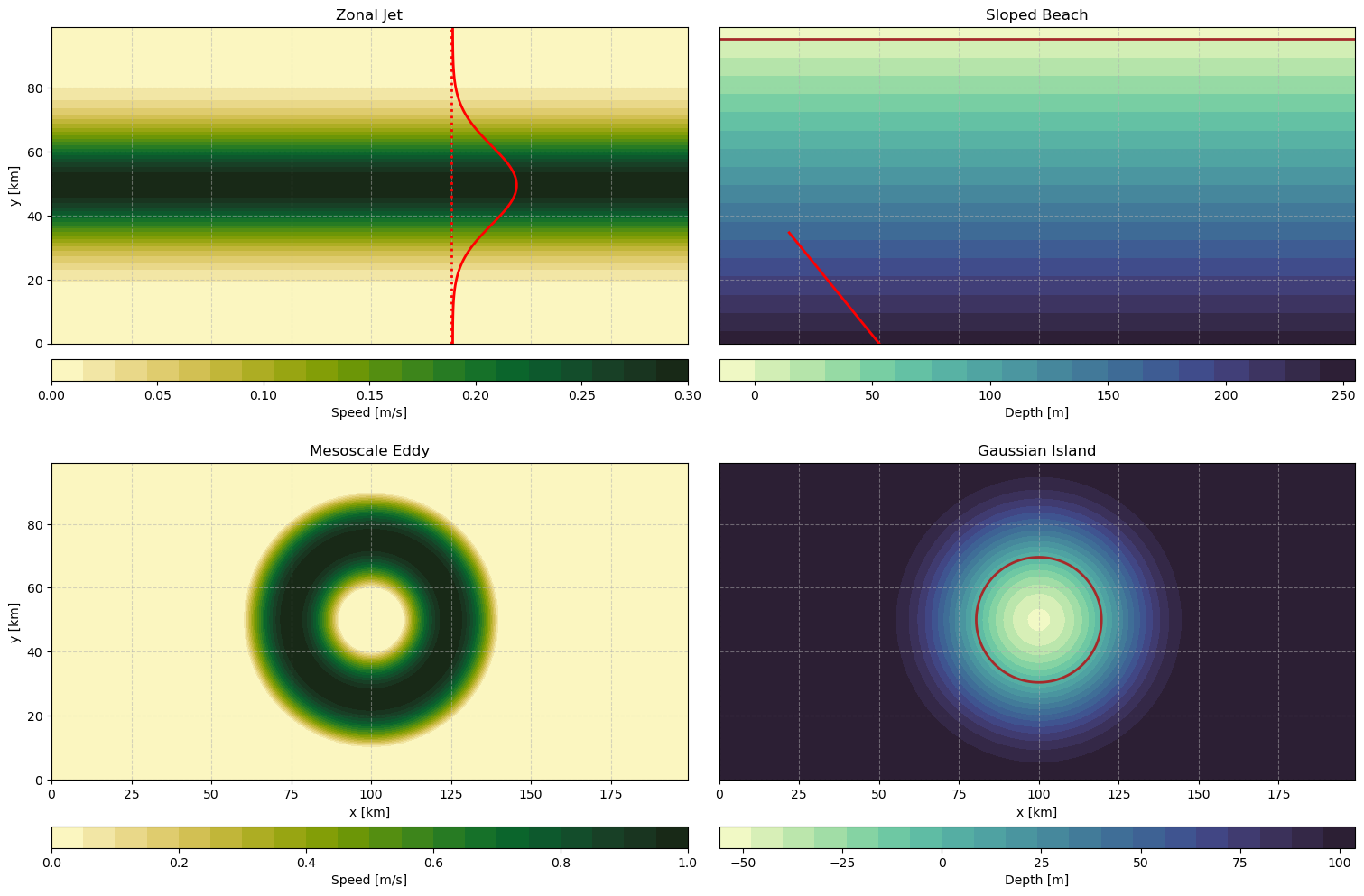
# Top left: zonal jet
cf_zj = axs[0, 0].contourf(x_km, y_km, zonal_speed, cmap=cmocean.cm.speed, levels=20)
axs[0, 0].axvline(125, color='red', linestyle=':', linewidth=2)
axs[0, 0].plot(profile_x, y_vals, color='red', linewidth=2)
axs[0, 0].set_title('Zonal Jet')
fig.colorbar(cf_zj, ax=axs[0, 0],
             orientation='horizontal', location='bottom',
             pad=0.02, shrink=1, aspect=30,
             label='Speed [m/s]',
             ticks=[0.0,0.05,0.1,0.15,0.2,0.25,0.3])

# Top right: beach
cf_beach = axs[0, 1].contourf(x_km, y_km, beach.depth, cmap=cmocean.cm.deep, levels=20)
axs[0, 1].contour(x_km, y_km, beach.depth, levels=[0], colors='brown', linewidths=2)
axs[0, 1].plot(line_x, line_y, color='red', linewidth=2)
axs[0, 1].set_title('Sloped Beach')
fig.colorbar(cf_beach, ax=axs[0, 1],
             orientation='horizontal', location='bottom',
             pad=0.02, shrink=1, aspect=30,
             label='Depth [m]',
             ticks=[0.0,50,100,150,200,250])

# Bottom left: mesoscale eddy
cf_eddy = axs[1, 0].contourf(x_km, y_km, eddy_speed, cmap=cmocean.cm.speed, levels=20)
axs[1, 0].set_title('Mesoscale Eddy')
fig.colorbar(cf_eddy, ax=axs[1, 0],
             orientation='horizontal', location='bottom',
             pad=0.02, shrink=1, aspect=30,
             label='Speed [m/s]',
             ticks=[0.0,0.2,0.40,0.6,0.8,1.0])

# Bottom right: gaussian island
cf_island = axs[1, 1].contourf(x_km, y_km, island.depth, cmap=cmocean.cm.deep, levels=20)
axs[1, 1].contour(x_km, y_km, island.depth, levels=[0], colors='brown', linewidths=2)
axs[1, 1].set_title('Gaussian Island')
fig.colorbar(cf_island, ax=axs[1, 1],
             orientation='horizontal', location='bottom',
             pad=0.02, shrink=1, aspect=30,
             label='Depth [m]',
             ticks=[-50,-25,0,25,50,75,100])

# Axis labels and settings
for ax in axs.flat:
    ax.set_aspect('equal')
    ax.grid(linestyle='--', alpha=0.5)

axs.flat[0].set_ylabel('y [km]')
axs.flat[2].set_ylabel('y [km]')
axs.flat[2].set_xlabel('x [km]')
axs.flat[3].set_xlabel('x [km]')

for ax in [axs.flat[0], axs.flat[1]]:
    ax.tick_params(axis='x', which='both', bottom=False, labelbottom=False)
for ax in [axs.flat[1], axs.flat[3]]:
    ax.tick_params(axis='y', which='both', left=False, labelleft=False)


# ---ANIMATION---
# Create empty line objects for rays in each panel
ray_lines_jet1 = [axs[0, 0].plot([], [], lw=0.8, color='black')[0] for i in range(bundle4jet.ray.size) if i % 2 == 0]
ray_lines_beach = [axs[0, 1].plot([], [], lw=0.8, color='white')[0] for i in range(bundle4beach.ray.size) if i % 2 == 0]
ray_lines_eddy = [axs[1, 0].plot([], [], lw=0.8, color='black')[0] for i in range(bundle4eddy.ray.size) if i % 2 == 0]
ray_lines_island = [axs[1, 1].plot([], [], lw=0.8, color='white')[0] for i in range(bundle4island.ray.size) if i % 2 == 0]

# Animation function
def animate(frame):
    for i, line in enumerate(ray_lines_jet1):
        ray = bundle4jet.isel(ray=2*i).sel(time_step=slice(0, frame))
        line.set_data(ray.x / 1e3, ray.y / 1e3)  # Convert to km

    for i, line in enumerate(ray_lines_beach):
        beach_frame = frame * 10  # or whatever slowdown factor you want
        ray = bundle4beach.isel(ray=2*i).sel(time_step=slice(0, beach_frame))
        line.set_data(ray.x / 1e3, ray.y / 1e3)

    for i, line in enumerate(ray_lines_eddy):
        ray = bundle4eddy.isel(ray=2*i).sel(time_step=slice(0, frame))
        line.set_data(ray.x / 1e3, ray.y / 1e3)

    for i, line in enumerate(ray_lines_island):
        ray = bundle4island.isel(ray=2*i).sel(time_step=slice(0, frame))
        line.set_data(ray.x / 1e3, ray.y / 1e3)

    return ray_lines_jet1 + ray_lines_beach + ray_lines_eddy + ray_lines_island

# Create the animation
anim = animation.FuncAnimation(
    fig, animate,
    frames=range(0, time_steps, 1),
    interval=40,
    blit=True
)

To show the animation, you can either a) use HTML to show it in the notebook (which will likely run into space issues) or b) save it as a gif. WARNING: This cell will take some time to output.

# To display in notebook, uncomment:
# HTML(anim.to_jshtml())

# To save to file:
anim.save("demo_animation.gif", writer=PillowWriter(fps=25))