Ray tracing in a Realistic Context: Nazare’s Canyon
import warnings
warnings.filterwarnings('ignore')

import numpy as np
import matplotlib.pyplot as plt

import xarray as xr
from PIL import Image
import requests
from io import BytesIO

import mantaray
import mantaray.datasets

from src import *
Introduction
This notebook tests the Ray Tracing Package with a realistic bathymetry and no current forcing.
Initialization:
Optical data are from the Sentinel-2 satellite available at: https://browser.dataspace.copernicus.eu. High resolution bathymetry data are from the European Commission and are available at https://emodnet.ec.europa.eu/
The initial conditions (wavelength, period, wavenumber, and direction) for the present example are obtained from spectral analysis of a Sentinel-2 image offshore Nazaré. The spectrum for that particular location, date, and time is available through the
mantaray.datasetsas “spec_s2.nc”.num_rays: is the number of rays the user would like to propagate. All rays have the same initial parametersx\(_{0}\), y\(_{0}\): are the locations initial positions of the rays
The flags
plot_spectrum,plot_bathyare for the users if they want to visualize in detail the wave spectrum from the Sentinel-2 image and the bathymetry.
# number of rays
num_rays = 100
plot_spectrum = True
plot_bathy = True
Load Sentinel-2 spectrum, brightness, and bathymetry from mantaray.datasets
#########
# Load Sentinel 2 spectrum
##########
spec_sentinel2_path = mantaray.datasets.fetch_spec_s2()
ds_spec_sentinel2 = xr.open_dataset(spec_sentinel2_path)
# Select wavenumber range to focus on the swell band
ds_spec_sentinel2 = ds_spec_sentinel2.sel(wavenumber =slice(0, 0.025))

#########
# Sentinel 2 image
##########
s2_nazare_path = mantaray.datasets.fetch_s2_image()
ds_s2_nazare = xr.open_dataset(s2_nazare_path)

#########
# Nazare Bathy
##########
nazare_depth_path = mantaray.datasets.fetch_nazare_bathy()
ds_nazare_depth = xr.open_dataset(nazare_depth_path)
variables = ['value_count', 'elevation']
ds_nazare_depth = ds_nazare_depth[variables]

ds_depth_meter_path = mantaray.datasets.fetch_bathy_nazare()
ds_depth_meter = xr.open_dataset(ds_depth_meter_path)
Vizualize the bathymetry and Sentinel-2 imagery
if plot_bathy:
    sub_nazare_S2fig, ax = plt.subplots()
    ds_s2_nazare.brightness.plot(vmin = 200, vmax = 1000, cmap = 'binary_r', add_colorbar = False)
    p2 = ax.pcolormesh(ds_nazare_depth.longitude+360, ds_nazare_depth.latitude, ds_nazare_depth.elevation, vmin = -500, vmax = 0, alpha = .6, cmap = 'Blues_r')
    cbar = plt.colorbar(p2)
    cbar.ax.set_ylabel('Depth [m]')
    ax.set_xlim([350.86, 350.95])
    ax.set_ylim([39.55, 39.62])
    ax.set_title('Bathymetry and Sentinel-2 imagery in the Nazare Region')

Define the initial location of rays based on the starting points (\(x_{0}\), \(y_{0}\))
#########
# --- The starting line for ray_tracing
#########
x_line = [45_000, 50_000]
y_line = [37_000, 40_000]

x_line_param = np.linspace(x_line[0], x_line[1], num_rays)
y_line_param = np.linspace(y_line[0], y_line[1], num_rays)

#########
# --- Loop through the points along the started line and find the closest pixels
#########
x0 = []
y0 = []
depth0 = []
XX, YY = np.meshgrid(ds_depth_meter.x.values, ds_depth_meter.y.values)
for x, y in zip(x_line_param, y_line_param):
    x_closest, y_closest, depth_closest = find_closest_pixel_depth(x, y, XX, YY,ds_depth_meter.depth.values)

    x0.append(float(x_closest))
    y0.append(float(y_closest))
    depth0.append(float(depth_closest))
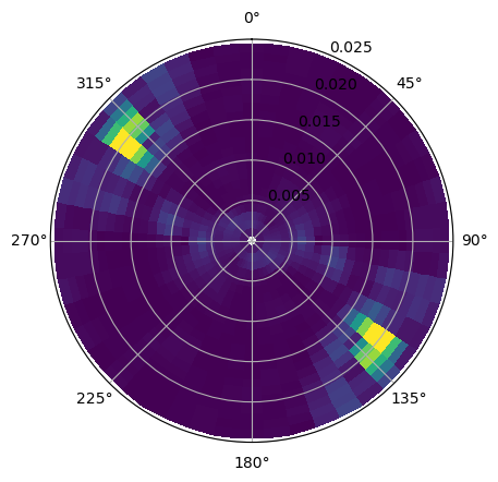
if plot_spectrum:
fig, ax = plt.subplots(subplot_kw = {'projection':'polar'})
ax.pcolormesh(ds_spec_sentinel2.directions, ds_spec_sentinel2.wavenumber, ds_spec_sentinel2.wave_directional_spectrum.T, vmin = 0, vmax = 2000)
ax.set_ylim([0, .025])
ax.set_theta_offset(np.pi/2) # shift the 0 to the nroth
ax.set_theta_direction(-1) # swap the direction (clockwise)
iddir, id_wn = np.where(ds_spec_sentinel2.wave_directional_spectrum.values == ds_spec_sentinel2.wave_directional_spectrum.values.max())
dp_spec = ds_spec_sentinel2.directions[iddir].values[0]*180/np.pi + 180 # swell cannot be from the coast (verified with the phase-difference spectrum)
lambda_p = (2*np.pi)/ds_spec_sentinel2.wavenumber[id_wn].values[0]
sigma = (g*ds_spec_sentinel2.wavenumber[id_wn].values[0])**(1/2)# intrinsic frequency
f = sigma/(2*np.pi)
T0 = 1/(f)
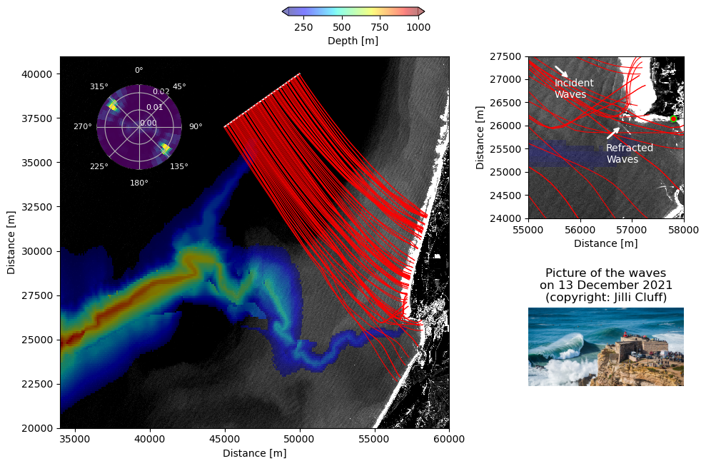
print(f'The incident wave direction is {dp_spec:.2f} deg and the wavelength is {lambda_p:.2f} m (T = {T0:.2f} sec)' )
The incident wave direction is 307.50 deg and the wavelength is 334.45 m (T = 14.64 sec)
Initialize the ray tracing with all the informations provided above
###########
# ---  Initial Wave Conditions
###########

k = 2*np.pi/lambda_p
depth = np.mean(depth0)
f = frequency_from_wavelength(lambda_p, depth)
cg = group_velocity(k, f, depth)
# Period of incident waves in seconds
T0 = 1/f
theta0 = dp_spec * np.pi/180
# Convert period to wavenumber magnitude
k0 = 2*np.pi/lambda_p

# Calculate wavenumber components
kx0 = k0*np.cos(theta0)
ky0 = k0*np.sin(theta0)


# Initialize wavenumber for all rays
Kx0 = kx0*np.ones(num_rays)
Ky0 = ky0*np.ones(num_rays)

# Current and bathymetry file path
# Note that the variable names have to be x, y, u, v, depth
current = mantaray.datasets.fetch_current_nazare()
bathymetry = ds_depth_meter_path

# Read x and y from file to get domain size
ds = xr.open_dataset(bathymetry)

# Estimates CFL
# Computes grid smallest spacing
dd = np.min([np.diff(ds.x).mean(), np.diff(ds.y).mean()])
# Computes group velocity in intermediate water
cg = group_velocity(k0, f, depth)
# Computes CFL
cfl = dd/cg

duration = round(x.max()/cg)
step_size = cfl
# Ray Tracing
bundle = mantaray.ray_tracing(x0, y0, Kx0, Ky0, duration, step_size, bathymetry, current)
Visualize rays
In this plot, we represent the wave rays based on the initial conditions provided previously in the notebook. One panel displays the regional domain, another displays a zoom around the Nazare’s peninsula. The wave spectrum computed from the Sentinel-2 image is provided in the plot. As an illustration of the waves from the coast, a picture taken from a photograph on the cliff on the day studied is displayed.
##########
# --- Longitude and Latitude meter steps -- for plot
##########
mean_lat = np.nanmean(ds_nazare_depth.latitude.values) # the mean latitude in the domain
delta_lon = abs(np.nanmean(np.diff(ds_nazare_depth.longitude)))
delta_lat = abs(np.nanmean(np.diff(ds_nazare_depth.latitude)))

# get the distance between two neighbouring pixels
dx_nazare_depth, dy_nazare_depth = decimal_coords_to_meters(delta_lon, delta_lat, mean_lat)

dx_sentinel_2 = 10 # this is from the sensor's parameter (/!\ don't change it /!\)
sub_s2_dist_x =(ds_s2_nazare.longitude.size)*dx_sentinel_2
sub_s2_dist_y =(ds_s2_nazare.latitude.size)*dx_sentinel_2

lon_meter_nazare_S2 = np.arange(0, sub_s2_dist_x, dx_sentinel_2)
lat_meter_nazare_S2 = np.arange(sub_s2_dist_y, 0, -dx_sentinel_2)

lon_meter_nazare_depth = np.arange(0, len(ds_nazare_depth.longitude.values)*dx_nazare_depth, dx_nazare_depth)
lat_meter_nazare_depth = np.arange(0, len(ds_nazare_depth.latitude.values) * dy_nazare_depth, dy_nazare_depth)
# --- For a beautiful plot, mask shallow waters
masked_depth = np.ma.masked_where(ds.depth.values<150, ds.depth.values)

fig = plt.figure(figsize=(10, 6))  # Adjust size as needed

# Define the grid dimensions and add subplots
ax1 = plt.subplot2grid((2, 3), (0, 0), rowspan=2, colspan=2)  # Large panel on the left
ax2 = plt.subplot2grid((2, 3), (0, 2))                       # Top-right panel
ax3 = plt.subplot2grid((2, 3), (1, 2))

ax_inset = fig.add_axes([.1, .7, .2, .2], projection = 'polar')

# --- Plot the wave directional spectrum
ax_inset.pcolormesh(ds_spec_sentinel2.directions, ds_spec_sentinel2.wavenumber, ds_spec_sentinel2.wave_directional_spectrum.T, vmin = 0, vmax = 2000)
ax_inset.set_ylim([0, .025])
ax_inset.set_theta_offset(np.pi/2) # shift the 0 to the nroth
ax_inset.set_theta_direction(-1) # swap the direction (clockwise)
ax_inset.tick_params(axis='both', which='both', colors='white', labelsize=8)
ax_inset.set_yticks([0, .01, .02])

# --- Plot the brightness observed by Sentinel-2 (panel (1))
ax1.pcolormesh(lon_meter_nazare_S2, lat_meter_nazare_S2, ds_s2_nazare.brightness,\
              vmin = 200, vmax = 1000, cmap = 'binary_r')
cs = ax1.pcolormesh(lon_meter_nazare_depth, lat_meter_nazare_depth, masked_depth, cmap = 'jet', vmin = 150, vmax = 1000, alpha = .5)
cax = fig.add_axes([.4, 1.06, 0.2, 0.02])
cbar = plt.colorbar(cs, cax = cax, orientation = 'horizontal', extend = 'both')
cbar.ax.set_xlabel('Depth [m]')
ax1.plot(x_line, y_line, color = 'w')

# --- Plot rays (panel (1))
for i in range(bundle.ray.size)[:]:
    ray = bundle.isel(ray=i)
    ax1.plot(ray.x, ray.y, 'r', lw=.78)

ax1.set_xlim([34_000, 60_000])
ax1.set_ylim([20_000, 41_000])
ax1.set_xlabel('Distance [m]')
ax1.set_ylabel('Distance [m]')

# --- Plot the brightness observed by Sentinel-2 (panel (2))

cs = ax2.pcolormesh(ds_depth_meter.x, ds_depth_meter.y, ds_depth_meter.depth)
ax2.pcolormesh(lon_meter_nazare_S2, lat_meter_nazare_S2, ds_s2_nazare.brightness,\
              vmin = 200, vmax = 1000, cmap = 'binary_r')
ax2.pcolormesh(lon_meter_nazare_depth, lat_meter_nazare_depth, masked_depth, cmap = 'jet', vmin = 150, vmax = 1000, alpha = .2)

start_inc = (55_500, 27_300)
end_inc = (55_800, 27_000)

start_ref = (56_500, 25_700)
end_ref = (56_800, 26_000)

ax2.annotate(
    '',  # No text
    xy=end_ref,  # End of the arrow
    xytext=start_ref,  # Start of the arrow
    arrowprops=dict(facecolor='white', edgecolor = 'white', arrowstyle='->', lw=2)  # Arrow properties
)
ax2.annotate(
    '',  # No text
    xy=end_inc,  # End of the arrow
    xytext=start_inc,  # Start of the arrow
    arrowprops=dict(facecolor='white', edgecolor = 'white', arrowstyle='->', lw=2)  # Arrow properties
)

ax2.text(56_500, 25_200, 'Refracted\nWaves', color = 'w')
ax2.text(55_500, 26_600, 'Incident\nWaves', color = 'w')
ax2.plot(57_800, 26_150, marker = 'o', markersize = 6,  color = 'lime')
ax2.plot(57_800, 26_150, marker = 'o', markersize = 4,  color = 'r')

# --- Plot rays (panel (2))
for i in range(bundle.ray.size)[:]:
    ray = bundle.isel(ray=i)
    ax2.plot(ray.x, ray.y, 'r', lw=.78)

ax2.set_xlim([55_000, 58_000])
ax2.set_ylim([24_000, 27_500])
ax2.set_xlabel('Distance [m]')
ax2.set_ylabel('Distance [m]')

# --- Plot(panel (3))
# URL of the image
url = "https://s3.amazonaws.com/www.explorersweb.com/wp-content/uploads/2021/12/14183820/hero-View-across-the-Fort-Nazare-lighthouse-Photo-RM-Nunes-via-Shutterstock.jpg"

# Fetch and load the image from the URL
response = requests.get(url)
img = Image.open(BytesIO(response.content))
ax3.imshow(img)  # Display the image in this panel
ax3.axis("off")  # Turn off axes for the image panel
ax3.set_title('Picture of the waves\non 13 December 2021\n(copyright: Jilli Cluff)')
plt.tight_layout()