Constructing Canonical Forcing Fields
from pathlib import Path

# data handling
import numpy as np
import xarray as xr

# plotting
import matplotlib.pyplot as plt
import cmocean

# helper functions
import utils
Introduction
This notebook will cover the synthesizing of the following forcing fields: 1) A homogeneous current field, 2) A zonal current jet, 3) A mesoscale eddy, 4) A constant bathymetry field, 5) and an idealized island.
With bonus files for a sloped beach.
All fields will be steady (no variation in time), a core assumption of the ray tracing equations.
output_dir = Path("forcing")
Domain Parameters
For these synthesized datasets, we will be using a 100 km by 200 km domain with 1 km grid spacing. Mantaray expects the grid to be in units of meters.
# Parameters for the background domain [m]
Lx = 200_000  # x-length
Ly = 100_000  # y-length
dx = 1_000  # x grid spacing
dy = 1_000  # y grid spacing
# x/y grid
x = np.arange(0, Lx, dx)
y = np.arange(0, Ly, dy)
xv, yv = np.meshgrid(x, y)
Currents
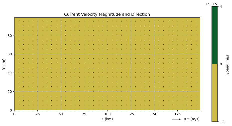
No Currents
This field will have the same u/v velocity (0 m/s) at all grid points and will be used for examples where we are interested in studying how the waves respond to different depth fields.
# Choose a u/v current speed [m/s]
u = 0
v = 0
# grid u/v
U_homog = np.full_like(xv, u)
V_homog = np.full_like(yv, v)
# build into an xarray dataset
ds_homog = xr.Dataset(
    data_vars={
        "x": (["x"], x),
        "y": (["y"], y),
        "u": (
            ["y", "x"],
            U_homog,
            {"long_name": "zonal current velocity", "units": "m/s"},
        ),
        "v": (
            ["y", "x"],
            V_homog,
            {"long_name": "meridional current velocity", "units": "m/s"},
        ),
    }
)
Note: data must be saved using the NETCDF3_CLASSIC format.
ds_homog.to_netcdf(output_dir / "homogeneous.nc", format="NETCDF3_CLASSIC")
# Plot using helper function
utils.plot_current_field(xv, yv, ds_homog, skip=5, q_scale=0.1)
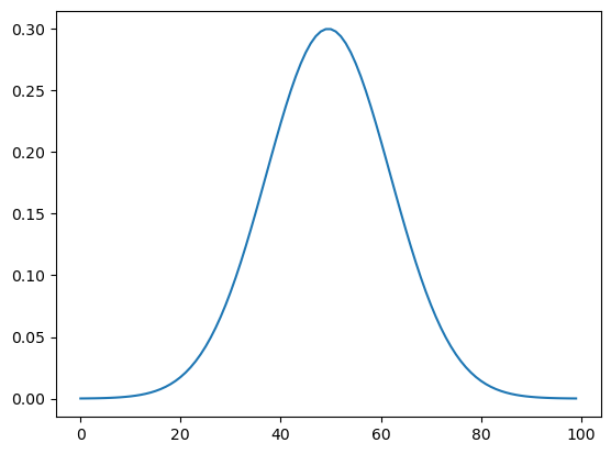
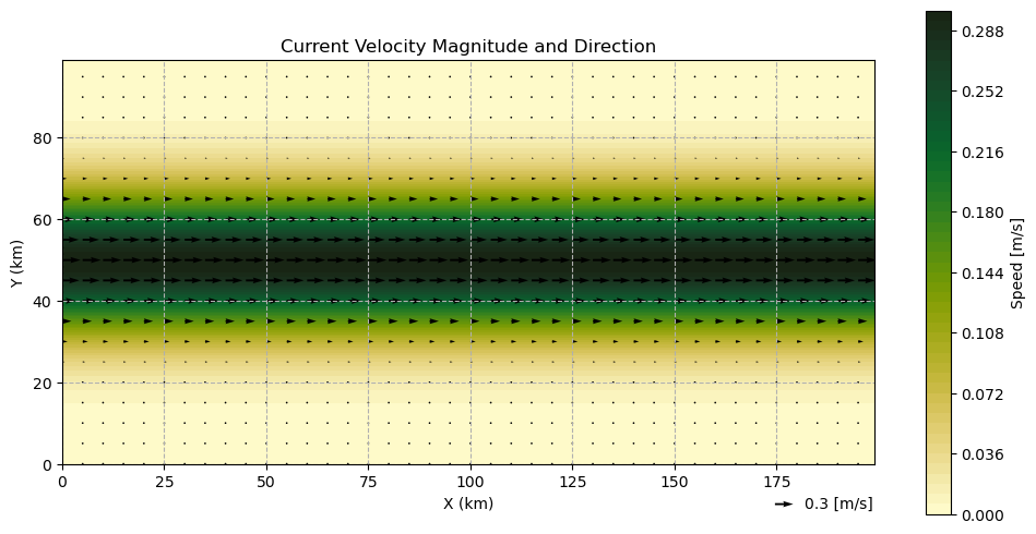
Zonal Jet
This field will have a zonal current jet whose profile follows a Gaussian distribution:
# Choose the maximum speed of the jet [m/s]
U_max = 0.3
width = 0.25  # controls how 'fat' the distribution (jet) is
x_profile = np.linspace(-1, 1, len(y))
U_profile = U_max * np.exp((-(x_profile**2)) / (2 * width**2))
plt.plot(U_profile)
[<matplotlib.lines.Line2D at 0x121cd8290>]
We extend the profile along the x-axis and assume there is no zonal current.
U_jet = np.ones((len(y), len(x))) * U_profile[:, np.newaxis]
V_jet = np.zeros_like(U_jet)
ds_jet = xr.Dataset(
    data_vars={
        "x": (["x"], x),
        "y": (["y"], y),
        "u": (
            ["y", "x"],
            U_jet,
            {"long_name": "zonal current velocity", "units": "m/s"},
        ),
        "v": (
            ["y", "x"],
            V_jet,
            {"long_name": "meridional current velocity", "units": "m/s"},
        ),
    }
)
ds_jet.to_netcdf(output_dir / "zonal_jet.nc", format="NETCDF3_CLASSIC")
utils.plot_current_field(xv, yv, ds_jet, skip=5, q_ref=0.3, q_scale=0.075)
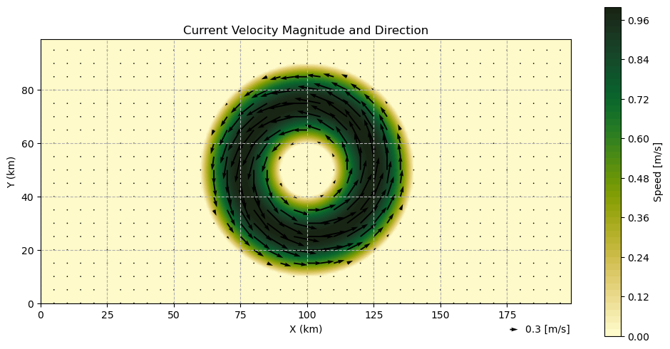
Mesoscale Eddy
We will construct a idealized parabolic mesoscale eddy following White and Fornberg 1997.
L_eddy = 80_000 # Diameter of the eddy [m]
R_eddy = L_eddy / 2
The number of grid points must be odd to ensure that the eddy is properly centered.
N = int(L_eddy / dx) + 1
Similar to our full domain, we make a smaller domain for the eddy.
# Create 2D grid
x_eddy = np.linspace(-R_eddy, R_eddy, N)
y_eddy = np.linspace(-R_eddy, R_eddy, N)

xv_eddy, yv_eddy = np.meshgrid(x_eddy, y_eddy)
We set the maximum speed of the Eddy to be 1 m/s to make it’s impact on rays more dramatic.
U_max = 1.0 # [m/s]
We will use a custom function to create a velocity field for a parabolic eddy as in White and Fornberg 1997.
u_eddy, v_eddy = utils.generate_parabolic_ring_eddy(L_eddy, U_max, xv_eddy, yv_eddy)
We now insert the eddy into a larger domain. We define the center of the eddy using the units of the domain.
# Define the center of the eddy [m]
center_x = 100_000
center_y = 50_000
Then, we can create a static background, find the indices of the center point, and insert the eddy.
# Create static background velocity field
u_background = np.zeros_like(xv).astype(float)
v_background = np.zeros_like(yv).astype(float)

idx_center_x = int((center_x - L_eddy / 2) / dx)
idx_center_y = int((center_y - L_eddy / 2) / dy)

# Insert the tapered eddy
u_background[
    idx_center_y : idx_center_y + len(x_eddy), idx_center_x : idx_center_x + len(x_eddy)
] += u_eddy
v_background[
    idx_center_y : idx_center_y + len(x_eddy), idx_center_x : idx_center_x + len(x_eddy)
] += v_eddy
ds_eddy = xr.Dataset(
    data_vars={
        "x": (["x"], x),
        "y": (["y"], y),
        "u": (
            ["y", "x"],
            u_background,
            {"long_name": "zonal current velocity", "units": "m/s"},
        ),
        "v": (
            ["y", "x"],
            v_background,
            {"long_name": "meridional current velocity", "units": "m/s"},
        ),
    }
)
ds_eddy.to_netcdf(output_dir / "mesoscale_eddy.nc", format="NETCDF3_CLASSIC")
utils.plot_current_field(xv, yv, ds_eddy, skip=5, q_ref=0.3, q_scale=0.05)
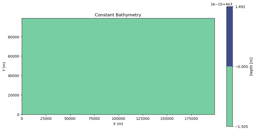
Constant Bathymetry
For the different current examples, we will use a constant deep bathymetry field.
bathy_const = np.full_like(xv, 4000) # [m]
ds_const = xr.Dataset(
    data_vars={
        "x": (["x"], x),
        "y": (["y"], y),
        "depth": (["y", "x"], bathy_const, {"long_name": "bathymetry", "units": "m"}),
    }
)
ds_const.to_netcdf(output_dir / "4000m_bathymetry.nc", format="NETCDF3_CLASSIC")
fig, ax = plt.subplots(figsize=(12, 6))

c = ax.contourf(xv, yv, bathy_const, cmap=cmocean.cm.deep)

fig.colorbar(c, ax=ax, label="Depth [m]")

ax.set_xlabel("X (m)")
ax.set_ylabel("Y (m)")

ax.set_title("Constant Bathymetry")

ax.set_aspect("equal")

plt.show()
Gaussian Island
We will also show an example of no currents but with an island sea mound.
# Island parameters [m]
L_mound = 1e5  # diameter of the sea mound
H_background = 100  # background depth
elevation = 50  # maximum height of the island (above sea level)
x_mound = np.arange(
    -L_mound / 2, L_mound / 2, dx
)  # x-axis values (symmetrical about 0)
y_mound = np.arange(
    -L_mound / 2, L_mound / 2, dy
)  # y-axis values (symmetrical about 0)
xv_mound, yv_mound = np.meshgrid(x_mound, y_mound)
R = np.sqrt(xv_mound**2 + yv_mound**2)

# Normalize the radial distance to range from 0 to L_x/2 (maximum radial distance)
R_normalized = np.clip(R / (L_mound / 2), 0, 1)  # Normalize radius, clip to [0, 1]

# Use sin^2 function to create the profile, with peak at sin^2(pi/2)
mound = (H_background + elevation) * np.sin(np.pi * R_normalized / 2 + np.pi / 2) ** 2
# Define island center in the larger bathymetry field
center_x = 100000  # meters
center_y = 50000  # meters
idx_center_x = int((center_x - L_mound / 2) / dx)
idx_center_y = int((center_y - L_mound / 2) / dy)

bathy_const = np.full_like(xv, H_background).astype(float)

# Subtract the island bump from the bathymetry field
bathy_island = bathy_const.copy()
bathy_island[
    idx_center_y : idx_center_y + len(y_mound),
    idx_center_x : idx_center_x + len(x_mound),
] -= mound
ds_island = xr.Dataset(
    data_vars={
        "x": (["x"], x),
        "y": (["y"], y),
        "depth": (["y", "x"], bathy_island, {"long_name": "bathymetry", "units": "m"}),
    }
)
ds_island.to_netcdf(output_dir / "gaussian_island.nc", format="NETCDF3_CLASSIC")
fig, ax = plt.subplots(figsize=(12, 6))

c = ax.contourf(xv, yv, bathy_island, cmap=cmocean.cm.deep, levels=50)

is_contour = ax.contour(xv, yv, bathy_island, levels=[0], colors="tan", linewidths=2)
is_contour = ax.contour(xv, yv, bathy_island, levels=[0], colors="tan", linewidths=2)


fig.colorbar(c, ax=ax, label="Depth [m]")

ax.set_xlabel("X (m)")
ax.set_ylabel("Y (m)")

ax.set_title("Constant Bathymetry")

ax.set_aspect("equal")

plt.show()
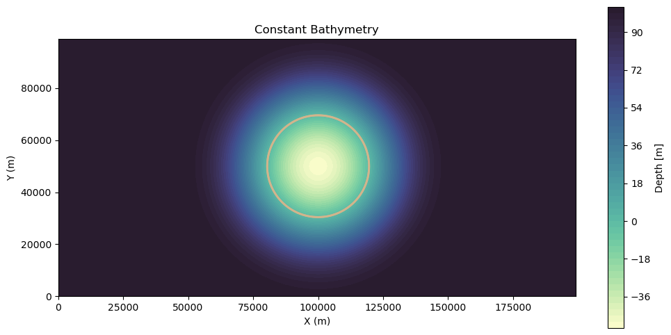
Note: following convention, more positive depth is deeper, while more negative depth is above sea level.
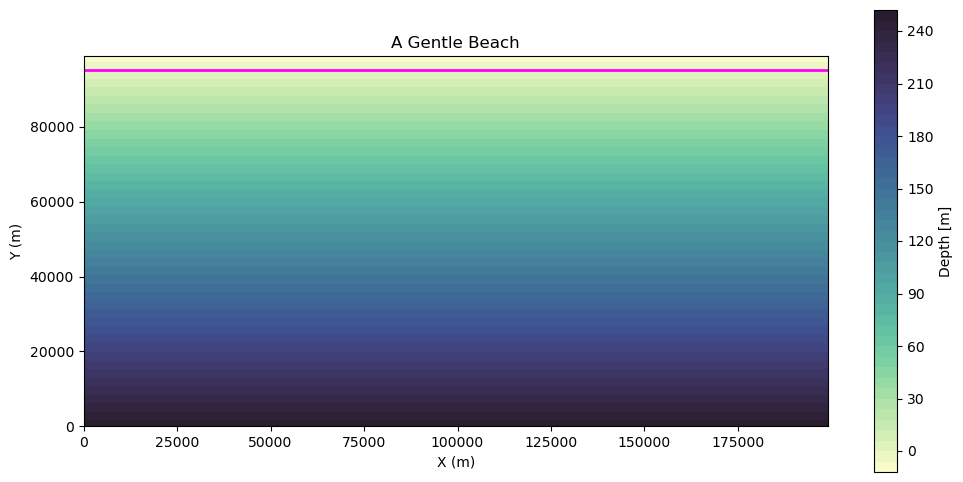
BONUS: A Gentle Beach
We will construct a bathymetry field that linearly increases in depth along the y-axis.
bathy_beach = np.tile(
    np.linspace(250, -10, yv.shape[0])[:, np.newaxis], (1, yv.shape[1])
)
ds_beach = xr.Dataset(
    data_vars={
        "x": (["x"], x),
        "y": (["y"], y),
        "depth": (["y", "x"], bathy_beach, {"long_name": "bathymetry", "units": "m"}),
    }
)
ds_beach.to_netcdf(output_dir / "gentle_slope.nc", format="NETCDF3_CLASSIC")
fig, ax = plt.subplots(figsize=(12, 6))

# Filled contour plot
c = ax.contourf(xv, yv, bathy_beach, cmap=cmocean.cm.deep, levels=50)

# Add contour line at 0 depth
zero_contour = ax.contour(
    xv, yv, bathy_beach, levels=[0], colors="magenta", linewidths=2
)

fig.colorbar(c, ax=ax, label="Depth [m]")

ax.set_xlabel("X (m)")
ax.set_ylabel("Y (m)")
ax.set_title("A Gentle Beach")

ax.set_aspect("equal")

plt.show()